Global definitions
At global level, a Chi program is a sequence of definitions, as shown in the following diagram.
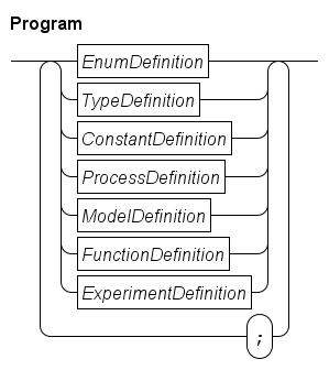
Each of the definitions is explained below. The syntax diagram suggests that a ; separator is obligatory between definitions. The implementation is more liberal, you may omit the separator when a definition ends with the end keyword. Also, it is allowed to use a separator after the last definition.
The name of each global definition has to be unique.
Enumeration definitions
With enumerations, you create a new enumeration type containing a number of names (called enumeration values). The syntax is given below.
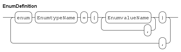
The enumeration definitions start with the keyword enum, followed by a sequence of definitions separated with a ,. Each definition associates an enumeration type name with a set of enumeration value names. For example:
enum FlagColours  = {red, white, blue},
     MachineState = {idle, heating, processing};
The enumeration type names act as normal types, and the enumeration values are its values. The values have to be unique words.
For example, you can create a variable, and compare values like:
MachineState state = idle;
...
while state != processing:
    ...
end
Note that enumeration values have no order, you cannot increment or decrement variables with an enumeration type, and you can only compare values with equality and inequality.
Type definitions
Type definitions allow you to assign a name to a type. By using a name instead of the type itself, readability of the program increases.
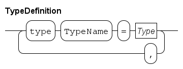
A type definition starts with the keyword type, followed by a number of 'assignments' that associate a type name with a type, separated with a ,. For further details about type names and types, see Types.
An example:
type lot   = real,
     batch = list lot;
Here a lot type name is introduced that is implemented with a real number, and a batch type name is created, which is a list of lot.
These type names can be used at every place where you can use a type, for example in variable declarations:
batch xs;
lot x;
Note that you cannot define use a type name in its own definition.
Constant definitions
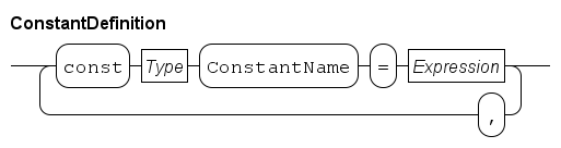
Constant definitions allow you to give a name to a fixed value to enhance readability. It also makes it easier to change a value between different experiments. For example, if you have a constant named speed, and you want to investigate how its value affects performance, you only have to change value in the constant definition, instead of finding and changing numbers in the entire program.
The syntax of constant definitions is as follows.
An example:
const real speed = 4.8,
      dict(string : list int) recipes = { "short" : [1,4,8],
                                          "long"  : [1,1,2,3,4,5] };
Here, a speed real value is defined, and recipes value, a dictionary of string to numbers. The constant names can be used at every point where you can use an expression. See the Expressions section for details about expressions.
Note that you cannot use a constant name in its own definition.
Process definitions
A process is an entity that shows behavior over time. A process definition is a template for such a process. It is defined as follows.
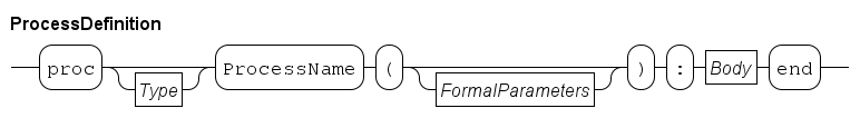
The definition starts with the keyword proc optionally followed by an exit type. The name of the process definition, and its formal parameters concludes the header. In the body, the behavior is described using statements.
Formal parameters are further explained in Formal parameters, statements are explained in the Statements section.
For example:
proc P():
  writeln("Hello");
  delay 15;
  writeln("Finished")
end
In the example, a process definition with the name P is defined, without parameters, that outputs a line of text when starting, and another line of text 15 time units later (and then finishes execution).
Creating and running a process is done with Sub-process statements (start or run) from another process or from a model.
If a process definition has no exit type specified, it may not use the exit statement, nor may it start other processes that have an exit type (see also Sub-process statements). Process definitions that have an exit type may use the exit statement directly (see Exit statement for details on the statement), and it may start other processes without exit type, or with the same exit type.
Since values returned by the exit statement may get printed onto the output, you may only use exit types that are printable. These are all the 'normal' data values, from simple booleans to lists, sets, and dictionaries of data values, but not channels, files, etc.
Model definitions
A model behaves like a process, the only difference is that a model is run as first process. It is the 'starting point' of a simulation. As such, a model can only take data values which you can write down as literal value. For example, giving it a channel or a process instance is not allowed.
Like the process, a model also has a definition. It is defined below.
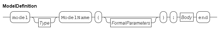
The syntax is exactly the same as process definitions explained in Process definitions, except it starts with a model keyword instead. A model can be started directly in the simulator (see Software operation), or as part of an experiment, explained in Simulating several scenarios, and Experiment definitions. If the model definition has no exit type, it may not use the exit statement directly, nor may it start other processes that have an exit type. If an exit type is specified, the model may use the exit statement to end the model simulation (see Sub-process statements for details), and it may start other processes, either without exit type, or with a matching exit type.
Function definitions
In programs, computations are executed to make decisions. These computations can be long and complex. A function definition attaches a name to a computation, so it can be moved to a separate place in the file.
Another common pattern is that the same computation is needed at several places in the program. Rather than duplicating it (which creates consistency problems when updating the computation), write it in a function definition, and call it by name when needed.
The syntax of a function definition is as follows.
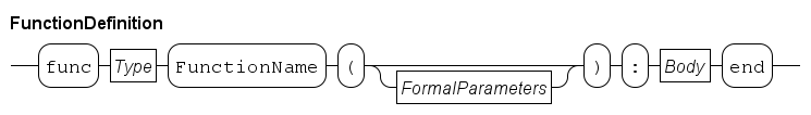
In the syntax, the only thing that changes compared with the syntax in Process definitions or Model definitions is the additional Type node that defines the type resulting from the computation.
However, since a function represents a computation (that is, calculation of an output value from input values) rather than having behavior over time, the Body part has additional restrictions.
A computation is performed instantly, no time passes. This means that you cannot delay or wait in a function.
A computation outputs a result. You cannot have a function that has no result.
A computation is repeatable. That means if you run the same computation again with the same input values, you get the same result every time. Also in the environment of the function, there should be no changes. This idea is known as mathematical functions.
A consequence of having mathematical functions is that you cannot interact with 'outside'. No querying of the current time, no communication, no select statement, and no use of distributions.
Technically, this would also imply no input/output, but for practical reasons this restriction has been lifted. However, as a general rule, avoid using it.
Experiment definitions
An experiment can execute one or more model simulations, collect their exit values, and combine them into a experiment result. Its syntax is shown below.
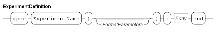
An experiment definition has some function-like restrictions, like not being able to use sub-process statements, no communication, and no use of time. On the other hand, it does not return a value, and it can start model simulations that have a non-void exit type (Void type discusses the void type).
The definition is very similar to other definitions. It starts with an xper keyword, followed by the name of the definition. The name can be used to start an experiment with the simulator (see Software operation for details on starting the simulator). If formal parameters are specified with the experiment definition (see Formal parameters below), the experiment can be parameterized with values. Like models, an experiment can only take data values which you can write down as literal value. For example, giving it a channel or a process instance is not allowed.
The body of an experiment is just like the body of a Function definitions (no interaction with processes or time). Unlike a function, an experiment never returns a value with the Return statement.
The primary goal of an xper is to allow you to run one or more model simulations that give an exit value. For this purpose, you can 'call' a model like a function, for example:
xper X():
    real total;
    int n;

    while n < 10:
        total = total + M();
        n = n + 1
    end

    writeln("Average is %.2f", total / 10);
end

model real M():
    dist real d = exponential(7.5);
    exit sample d;
end
The model above is very short to keep the example compact. In practice it will be larger, start several concurrent processes, and do a lengthy simulation before it decides what the answer should be. The experiment X makes ten calls to the model. Each call causes the model to be run, until the model or one of its processes executes the exit statement. At that point, the model and all its processes are killed, and the value supplied with the exit statement becomes the return value of the model call, adding it to total. After the ten model simulations, the experiment outputs the average value of all model simulations.
Note that the called model (or one of its started processes) must end with the exit statement, it is an error when the model ends by finishing its last model statement.
Formal parameters
Definitions above often take values as parameter to allow customizing their behavior during execution. The definition of those parameters are called formal parameters. The syntax of formal parameters is shown below.
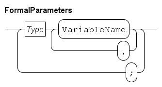
As you can see, they are just variable declarations (explained in the Local variables section), except you may not add an initial value, since their values are obtained during use of the definition.
To a definition, the formal parameters act like variables. You may use them just like other variables.
An example, where int x, y; string rel are the formal parameters of process definition P:
proc P(int x, y; string rel):
    writeln("%d %s %d", x, rel, x-y)
end

...

run P(2, -1, "is less than");
The formal parameters introduce additional variables in the process, that can be just like any other variable. Here, they are just printed to the screen. Elsewhere in the program, the definition gets used (instantiated), and a value is supplied for the additional variables. Such values are called actual parameters.