RasterFrames: Enabling DataFrame-Based Analysis of Big Spatiotemporal Raster Data

Background

Human beings have a millennia-long history of organizing information in tabular form. Typically, rows represent independent events or observations, and columns represent measurements from the observations. The forms have evolved, from hand-written agricultural records and transaction ledgers, to the advent of spreadsheets on the personal computer, and on to the creation of the DataFrame data structure as found in R Data Frames and Python Pandas. The table-oriented data structure remains a common and critical component of organizing data across industries, and is the mental model employed by many data scientists across diverse forms of modeling and analysis.

Today, DataFrames are the lingua franca of data science. The evolution of the tabular form has continued with Apache Spark SQL, which brings DataFrames to the big data distributed compute space. Through several novel innovations, Spark SQL enables interactive and batch-oriented cluster computing without having to be versed in the highly specialized skills typically required for high-performance computing. As suggested by the name, these DataFrames are manipulatable via standard SQL, as well as the more general-purpose programming languages Python, R, Java, and Scala.

RasterFrames®, an incubating Eclipse Foundation LocationTech project, brings together Earth-observing (EO) data analysis, big data computing, and DataFrame-based data science. The recent explosion of EO data from public and private satellite operators presents both a huge opportunity as well as a challenge to the data analysis community. It is Big Data in the truest sense, and its footprint is rapidly getting bigger. According to a World Bank document on assets for post-disaster situation awareness [^1]:

Of the 1,738 operational satellites currently orbiting the earth (as of 9/[20]17), 596 are earth observation satellites and 477 of these are non-military assets (ie available to civil society including commercial entities and governments for earth observation, according to the Union of Concerned Scientists). This number is expected to increase significantly over the next ten years. The 200 or so planned remote sensing satellites have a value of over 27 billion USD (Forecast International). This estimate does not include the burgeoning fleets of smallsats as well as micro, nano and even smaller satellites... All this enthusiasm has, not unexpectedly, led to a veritable fire-hose of remotely sensed data which is becoming difficult to navigate even for seasoned experts.

RasterFrames provides a DataFrame-centric view over arbitrary EO data, enabling spatiotemporal queries, map algebra raster operations, and compatibility with the ecosystem of Spark ML algorithms. By using DataFrames as the core cognitive and compute data model, it is able to deliver these features in a form that is accessible to general analysts while handling the rapidly growing data footprint.

Architecture

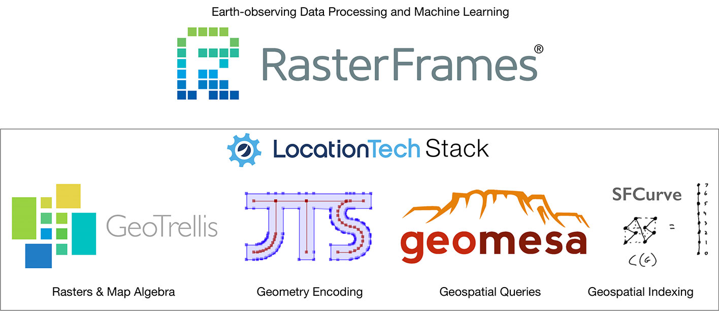
RasterFrames takes the Spark SQL DataFrame and extends it to support standard EO operations. It does this with the help of several other LocationTech projects: GeoTrellis, GeoMesa, JTS, and SFCurve.

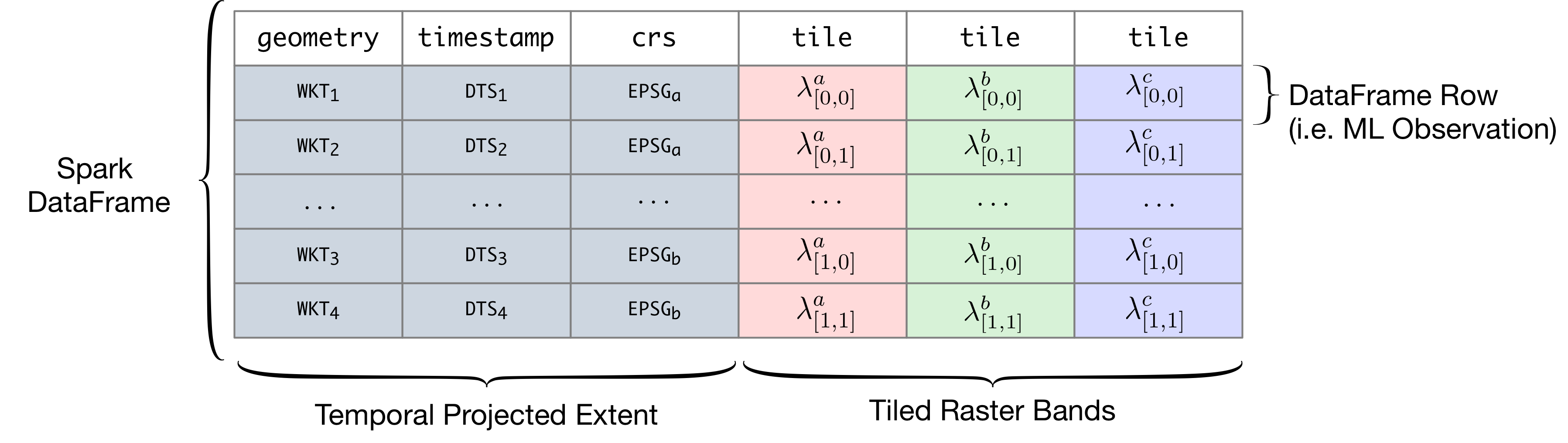
RasterFrames introduces a new native data type called tile to Spark SQL. Each tile cell contains a 2-D matrix of "cell" (pixel) values, along with information on how to numerically interpret those cells. A "RasterFrame" is a Spark DataFrame with one or more columns of type tile. A tile column typically represents a single frequency band of sensor data, such as "blue" or "near infrared", discretized into regular-sized chunks, but can also be quality assurance information, land classification assignments, or any other discretized geo-spatiotemporal data. It also includes support for working with vector data, such as GeoJSON. Along with tile columns there is typically a geometry column (bounds or extent/envelope) specifying the location of the data, the map projection of that geometry (crs), and a timestamp column representing the acquisition time. These columns can all be used in the WHERE clause when querying a catalog of imagery.

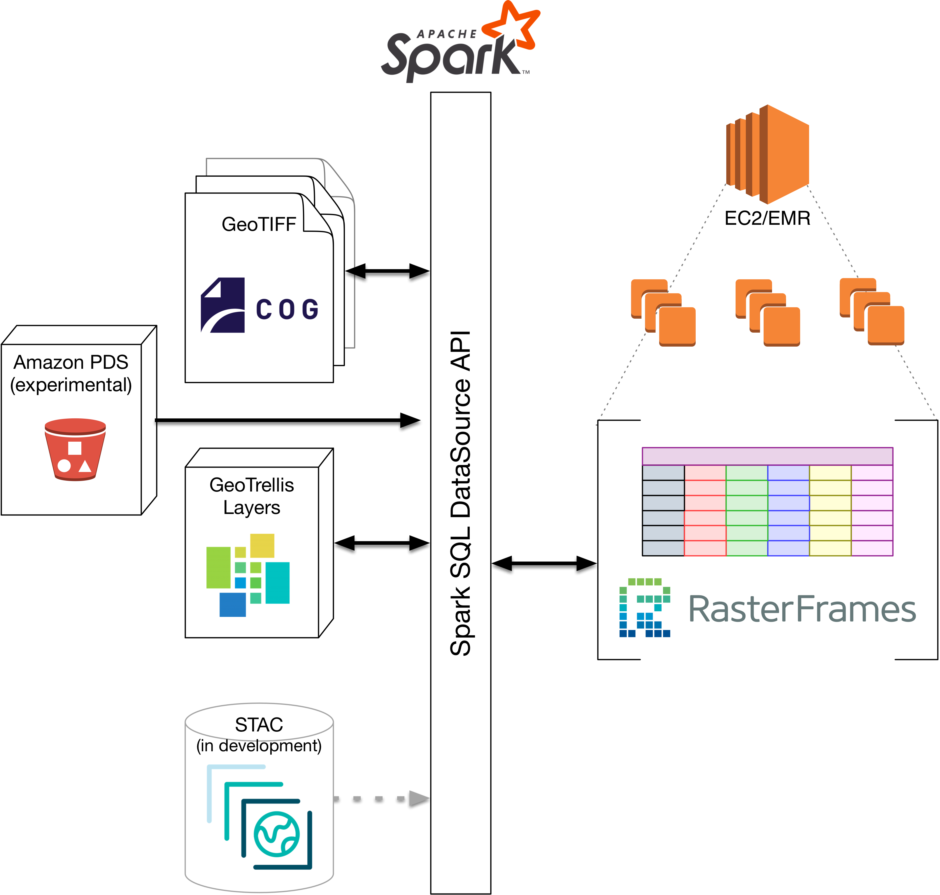
Raster data can be read from a number of sources. Through the flexible Spark SQL DataSource API, RasterFrames can be constructed from collections of (preferably Cloud Optimized) GeoTIFFs, GeoTrellis Layers, and from an experimental catalog of Landsat 8 and MODIS data sets on the Amazon Web Services (AWS) Public Data Set (PDS). We are also experimenting with support for the evolving Spatiotemporal Asset Catalog (STAC) specification.

Using RasterFrames

The following example shows some of the general operations available in RasterFrames. As an imagery target we will use the MODIS Nadir BRDF-Adjusted Surface Reflectance Data Product from NASA, which is available as GeoTIFFs through AWS PDS. The example extracts data using the RasterFrames MODIS catalog data source and manipulates it via SQL (as noted above, Python, Java, and Scala are also options). We will compute the monthly global average of a vegetation index in 2017 and see how it varies over the year.

Note: RasterFrames version 0.8.0-RC1 was used in this example.

The first step is to load the MODIS catalog data source into a table and take a look a the schema:

CREATE TEMPORARY VIEW modis USING `aws-pds-modis`;
DESCRIBE modis;
-- +----------------+------------------+
-- |col_name        |data_type         |
-- +----------------+------------------+
-- |product_id      |string            |
-- |acquisition_date|timestamp         |
-- |granule_id      |string            |
-- |gid             |string            |
-- |assets          |map<string,string>|
-- +----------------+------------------+

The assets column contains a dictionary mapping band names to URIs holding the location of each GeoTIFF. To determine what bands are available in the catalog we execute the following:

SELECT DISTINCT explode(map_keys(assets)) as asset_keys
FROM modis
ORDER BY asset_keys
-- +-------------+
-- |   asset_keys|
-- +-------------+
-- |          B01|
-- |        B01qa|
-- |          B02|
-- |        B02qa|
-- |          ...|
-- +-------------+

From the data product's user manual we find that B01 and B02 assets map to the red and NIR bands. From there we create a query reading the red and NIR band data on the (arbitrarily chosen) 15th of each month in 2017. This will give us 12 global coverages from which we will compute our statistics.

CREATE TEMPORARY VIEW red_nir_tiles_monthly_2017 AS
SELECT granule_id, month(acquisition_date) as month, 
       f_read_tiles(assets['B01'], assets['B02']) as (crs, extent, red, nir)
FROM modis
WHERE year(acquisition_date) = 2017 AND day(acquisition_date) = 15;
DESCRIBE red_nir_tiles_monthly_2017;
-- +--------+-------------------------------------------------------+
-- |col_name|data_type                                              |
-- +--------+-------------------------------------------------------+
-- |month   |int                                                    |
-- |crs     |struct<crsProj4:string>                  		    |
-- |extent  |struct<xmin:double,ymin:double,xmax:double,ymax:double>|
-- |red     |tile                                                   |
-- |nir     |tile                                                   |
-- +--------+-------------------------------------------------------+

Computing the normalized difference vegetation index (NDVI) is a very common operation in EO analysis, and is calculated simply as the normalized difference of the Red and NIR bands from a surface reflectance data product:

Since a normalized difference is such a common operation in EO analysis, RasterFrames includes the function rf_normalizedDifference to compute it. For this example we first compute NDVI and then collect the aggregate statistics (via rf_aggStats) on a per-month basis:

SELECT month, ndvi_stats.* FROM (
    SELECT month, rf_aggStats(rf_normalizedDifference(nir, red)) as ndvi_stats
    FROM red_nir_tiles_monthly_2017
    GROUP BY month
    ORDER BY month
)
-- +-----+---------+-----------+----+---+-------------------+-------------------+
-- |month|dataCells|noDataCells|min |max|mean               |variance           |
-- +-----+---------+-----------+----+---+-------------------+-------------------+
-- |1    |530105436|1261254564 |-1.0|1.0|0.2183160845625243 |0.12890947667168529|
-- |2    |600524070|1213875930 |-1.0|1.0|0.19716944997032773|0.12721311415470044|
-- |3    |615820993|1198579007 |-1.0|1.0|0.20199490649244112|0.12937148422536485|
-- |4    |629659958|1138660042 |-1.0|1.0|0.24221570883272578|0.13896602048542867|
-- |5    |635920714|1074799286 |-1.0|1.0|0.2949905328774185 |0.15610215565162433|
-- |6    |617826616|1092893384 |-1.0|1.0|0.3430829566130305 |0.1768520590388395 |
-- |7    |604436464|1106283536 |-1.0|1.0|0.37280247950373924|0.19128743861294956|
-- |8    |598500660|1169819340 |-1.0|1.0|0.3620362092401007 |0.19355049617163744|
-- |9    |623849120|1190550880 |-1.0|1.0|0.30889448330373964|0.1727205792001795 |
-- |10   |613413505|1200986495 |-1.0|1.0|0.2771316767269186 |0.15228789046594618|
-- |11   |546679019|1244680981 |-1.0|1.0|0.2510236308996954 |0.1348450714383397 |
-- |12   |520511978|1201728022 |-1.0|1.0|0.237714687195611  |0.13236712076432644|
-- +-----+---------+-----------+----+---+-------------------+-------------------+

Plotting the resultant mean value and standard deviation bands shows the following:

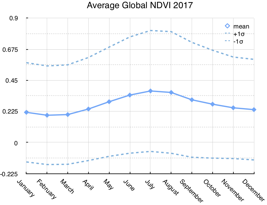
(While the curve is interesting, interpreting it is beyond the scope of this article.)

This is but a simple example of what one can do with RasterFrames. In the documentation we provide other examples, including supervised and unsupervised machine learning, as well as options for rendering results as new imagery layers.

Scalability

As stated in the introduction, a primary benefit of RasterFrames is its ability to scale with additional compute hardware. This means that not only can we attempt analyses that extend beyond the bounds of a single computer, but that we can also trade money for time. The example above was run 6 times using different sized Elastic Map Reduce (EMR) clusters on AWS. A modest node size (AWS "m4.large") was used, each composed of 4 virtual cores, 8 GB RAM, and 32 GB HDD.

Nodes	Cores	Memory (GB)	Execution Time (min)
1	4	8	80
3	12	24	27
5	20	40	18
7	28	56	12
11	44	88	9
15	60	120	8

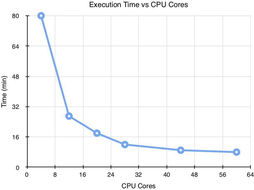
In this particular job we achieved significant scalability up until about 11 nodes. Cursory analysis indicated that the limiting factor in this analysis was network saturation. Analyses with greater computational requirements (say, K-means clustering), would be better able to make use of even more hardware.

At the time of writing, all 6 jobs cost less than the price of a cup of coffee, making it very much within the reach of any business user.

Conclusion

As more and more data becomes available in every industry, solutions have emerged to connect the traditional, tabular model of data to computational engines powerful enough to process it at volume. DataFrames and Spark SQL are general purpose tools that provide scalable data analysis through distributed computing. Data science and machine learning are consistently becoming more mainstream, and there is an opportunity for specialized technologies to further abstract common constructs within each problem space. For the EO realm, RasterFrames adds another layer of abstraction that can empower a broader set of users to process EO data in an intuitive way. By combining the technological advancements of its fellow Tech projects with DataFrames and Spark SQL, RasterFrames unlocks more natural, scalable machine learning for data analysts and scientists operating under a flood of new data while attempting to address global issues such as deforestation, climate change, and food shortages. As an open-source project and a proud member of Eclipse LocationTech, RasterFrames strives to have a positive global impact.

Learn More

To try out RasterFrames we recommend starting out with the preconfigured Docker image containing Jupyter Notebooks. A library of examples in both Python and Scala are included. Additional examples and details on doing development with RasterFrames on the RasterFrames website rasterframes.io.